spxtacular

spxtacular is a Python library for mass-spectrum processing: denoising, isotope deconvolution, charge assignment, matching, scoring, and interactive visualization behind one chainable Spectrum object. It's for anyone writing proteomics, metabolomics, lipidomics, glycomics, or oligonucleotide analysis code who wants raw peaks in and clean, annotated results out without hand-rolling the signal processing.

Part of the tacular-omics ecosystem alongside peptacular, paftacular, and mzmlpy.

Why spxtacular?

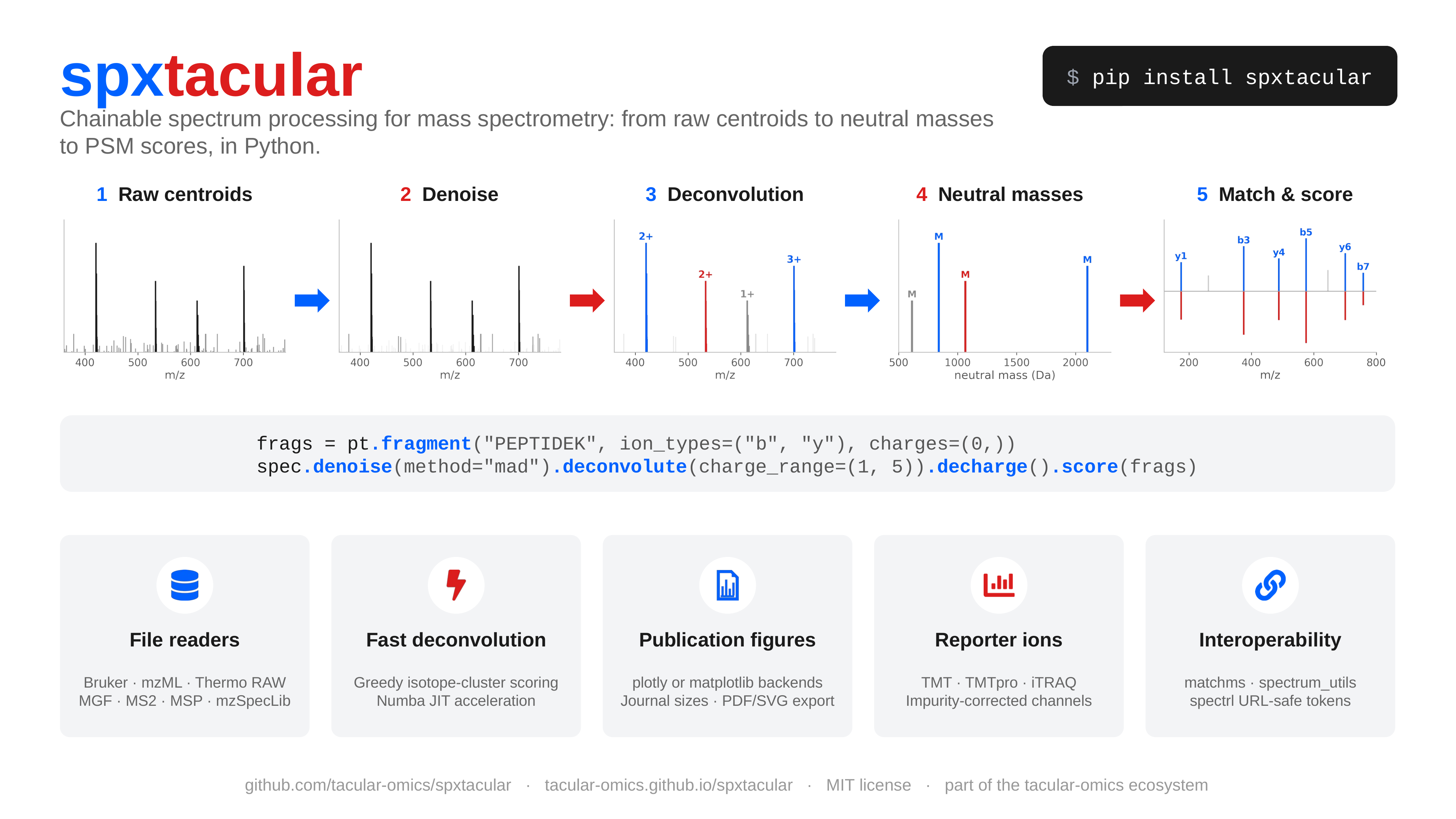
• One chainable API for the whole pipeline — denoise, deconvolute, decharge, match, score, and plot — that works the same for peptides, lipids, glycans, and nucleic acids.
• Reads what your instrument wrote. Reader auto-detects Bruker timsTOF .d, mzML, and Thermo .raw from the path, including gzipped and disk-backed mzML.
• Accessible visualization by default — a colour-vision-safe palette validated in light and dark mode, plus an HTML table_view() for screen readers, not an afterthought extra.
• Analyte-aware deconvolution — built-in isotope models for peptides, lipids, glycans, and nucleic acids, plus adduct-aware neutral-mass conversion ([M+H]+, [M-H]-, [M+Na]+, custom).
• Plays well with the ecosystem — lazy, optional bridges to matchms and spectrum_utils, and compact URL-safe spectrl tokens for sharing a spectrum with no backend.

Install

pip install spxtacular

# Optional: Numba JIT acceleration
pip install spxtacular[numba]

# Optional: share spectra as compact URL-safe tokens (spectrl)
pip install spxtacular[spectrl]

# Optional: raw-file readers — Bruker .d, mzML, Thermo .raw
pip install spxtacular[bruker]      # tdfpy — DReader
pip install spxtacular[mzml]        # mzmlpy — MzmlReader
pip install spxtacular[thermo]     # fisher-py — ThermoReader (also needs a .NET runtime)
pip install spxtacular[readers]     # all three readers

# Optional: publication figures (matplotlib backend) and static export of plotly figures
pip install spxtacular[matplotlib]
pip install spxtacular[plotly-export]

# Everything (numba + readers + spectrl + interoperability adapters + figure backends)
pip install spxtacular[all]

Quick start

import numpy as np
import spxtacular as spx

# A 2+ envelope near m/z 500 and a 3+ envelope near m/z 801, over a noise floor.
mz = np.array([
    352.1100, 418.4400, 476.9200,
    500.2573, 500.7590, 501.2606,
    655.3100, 733.0800,
    801.3073, 801.6417, 801.9762, 802.3106,
    918.6500, 1102.4000,
])
intensity = np.array([
    820.0, 1350.0, 690.0,
    100000.0, 51973.0, 11066.0,
    1580.0, 1015.0,
    52335.0, 60000.0, 34070.0, 12544.0,
    745.0, 1240.0,
])

spec = spx.Spectrum(mz=mz, intensity=intensity)

# Full pipeline: denoise → deconvolute → neutral mass
neutral = (
    spec
    .denoise(method="mad")
    .deconvolute(charge_range=(1, 5), tolerance=15, tolerance_unit="ppm", min_score=0.4)
    .decharge()
)

for peak in neutral.peaks:
    print(peak)
# Peak(mz=998.5000, int=1.52e+05, z=0, score=1.000)
# Peak(mz=2400.8999, int=1.46e+05, z=0, score=0.998)

neutral.plot(title="Neutral masses").show()

Reading raw files works the same for every format — Reader picks DReader, MzmlReader, or ThermoReader from the path suffix:

with spx.Reader("run.mzML") as reader:   # or spx.Reader("/data/sample.d") / spx.Reader("run.raw")
    print(reader.access_strategy)         # embedded, rapidgzip, memory, stream, plain, or None
    for spec in reader.ms1:              # .ms1/.ms2 are iterable *and* indexable
        ...

Gzipped mzML uses automatic disk-backed access by default. Create a self-indexed gzip artifact with spx.write_indexed_mzml_gzip("run.mzML", "run.indexed.mzML.gz").

Features

Feature	Description
Isotope deconvolution	Adaptive BRAIN envelopes, apex-first missing-mono recovery, biological/custom models, and optional Numba acceleration
Quality filtering	min_score, m/z, intensity, charge, and ion mobility filters
Neutral mass conversion	decharge() converts charged clusters to neutral masses
Fragment matching	match_fragments() with ppm/Da tolerance
PSM scoring	Hyperscore, spectral angle, matched fraction, and more
Interactive visualization	Stick, mirror, faceted, mass-error, and annotated fragment plots (Plotly), plus a sequence coverage ladder
Accessible by design	Colour-vision-safe palette validated in light and dark modes (spxtacular.theme), relative-intensity y-axis by default, capped/collision-avoided labels, and table_view() for a screen-reader-friendly peak table
File reading	Bruker timsTOF .d files (DReader), mzML (MzmlReader), and Thermo .raw (ThermoReader, vendor centroids included), or Reader to auto-detect the format from the path
Peak lists & libraries	Read and write MGF, MS2, and MSP spectral libraries (MgfReader, Ms2Reader, MspReader + matching writers) — pure standard library, gzip-aware, no extra to install
JSON transport	Versioned, class-preserving JSON round-trips for Spectrum, MsnSpectrum, and Chromatogram, with packaged JSON Schema documents
Spectrum sharing	Encode a full spectrum to a compact, URL-safe spectrl token or link (to_spectrl_token / to_spectrl_url)

Deconvolution pipeline

# 1. Find isotope clusters → assign monoisotopic m/z + charge + Bhattacharyya score
decon = spec.deconvolute(charge_range=(1, 5), tolerance=10, tolerance_unit="ppm")

# charge > 0  → assigned cluster
# charge = -1 → singleton / unassigned
# score 0–1   → isotope profile quality (0.0 for singletons)

# 2. Keep only high-confidence clusters
filtered = decon.filter(min_score=0.5)

# 3. Convert to neutral masses (drops singletons)
neutral = filtered.decharge()

Choose an average-composition model for the analyte class, or supply a custom IsotopeModel. Peptides remain the default for backward compatibility:

lipid_neutral = spec.deconvolute(
    isotope_model="lipid",
    ionization_model="[M+Na]+",
).decharge()

Polarity and adducts are explicit while charge arrays remain positive magnitudes: ionization_model="[M-H]-" or "[M+Na]+" covers common adducts, and a custom IonizationModel handles the rest. See Deconvolution for the full model list and how to write your own.

Visualization

Every figure is described once and drawn by either backend: plotly for interactive work (the default) or matplotlib for print. Three styles size the text and lines for the medium ("paper", "screen", "talk"), and size= takes journal column widths. Ion labels are typeset (y₇²⁺, b₅−H₂O), coloured by series and placed so they never overlap. Colours come from one theme module, checked for colour-vision deficiency in light and dark mode.

import peptacular as pt
import spxtacular as spx

frags = pt.fragment("PEPTIDE", ion_types=("b", "y"), charges=(1, 2))

fig = spec.annotate(frags)                                   # interactive plotly figure
spx.save_figure(fig, "spectrum.html")

# A journal figure: one column wide, 7 pt Arial, vector PDF with embedded fonts
fig = spx.annotate_spectrum(spec, frags, peptide="PEPTIDE", mass_error_panel=True,
                            backend="matplotlib", style="paper", size="single")
spx.save_figure(fig, "figure2.pdf")

# Several panels, lettered a-d, at full page width
parts = [spx.annotate_spectrum(spec, frags, backend="spec"),
         spx.mirror_plot(query, library, fragments=frags, similarity="cosine", backend="spec"),
         spx.sequence_coverage_plot(spec, "PEPTIDE", frags, backend="spec"),
         spx.reporter_ion_plot(spec, "TMT10", backend="spec")]
spx.save_figure(spx.compose_figure(parts, ncols=2), "figure3.pdf")

html = spx.table_view(spx.build_annot_plot_table(spec, frags))  # accessible table

docs/gallery/build.py renders every figure type in both backends.

matchms and spectrum_utils

Install spxtacular[matchms], spxtacular[spectrum-utils], or spxtacular[interop] for both. The integrations are lazy optional adapters, so the base package does not import either stack.

import spxtacular as spx

# matchms pipelines, similarities, Spec2Vec, MS2DeepScore, etc.
matchms_spec = spx.to_matchms(spec, extra_metadata={"smiles": "CCO"})
restored = spx.from_matchms(matchms_spec)

# spectrum_utils ProForma annotation and Matplotlib / Altair plots
su_spec = spx.to_spectrum_utils(ms2_spec)
su_spec.annotate_proforma("PEPTIDE/2", 10, "ppm")

The matchms bridge stable-sorts peaks and includes conventional metadata plus a namespaced payload that preserves spxtacular's richer fields on return conversion. The spectrum_utils bridge is necessarily lossy: its model holds one precursor and no per-peak charge, ion mobility, isotope score, or acquisition metadata. It warns when populated fields are dropped, and its upstream model stores intensities as float32.

Sharing spectra

With the optional [spectrl] extra, encode a complete spectrum (peaks, charges, ion mobility, and MSn metadata) into a single compact, URL-safe token — or a ready-to-share link — with no backend required.

token = spec.to_spectrl_token()                       # spectrl.v3.… token
restored = spx.Spectrum.from_spectrl_token(token)

url = spec.to_spectrl_url(base="https://example.com/view")  # …#spectrl.v3.… (shareable)
restored = spx.Spectrum.from_spectrl_url(url)

Isobaric reporter ions

TMT, TMTpro and iTRAQ reporter intensities, with channels and m/z from tacular and optional isotope impurity correction from the reagent lot sheet:

ions = spec.reporter_ions("TMT10")          # most intense peak within 20 ppm per channel
ions.intensity, ions.ppm_error

lot = {"126": {"-2": 0.0, "-1": 0.0, "+1": 7.0, "+2": 0.2}, ...}   # from the lot sheet
table = spx.reporter_ion_table(reader.ms2, "TMTpro18", impurities=lot, normalize="sum")

Documentation

Full documentation with API reference, guides, and interactive plots is available at tacular-omics.github.io/spxtacular.

• Spectrum API
• Deconvolution
• Readers
• Matching, scoring & reporter ions
• Visualization
• API Reference

Citing and contributing

Citation metadata is available in CITATION.cff. All archived releases are available from Zenodo at doi:10.5281/zenodo.19342437. See the changelog for release notes. Bug reports, support questions, and contributions are welcome; see CONTRIBUTING.md for the development workflow and community guidelines.

License

MIT