Advancements in computer processing power has opened a new area of using computer vision within autonomous vehicles. Computer vision techniques are designed to operate using visible light cameras to perform specific task much like humans do. Examples of current uses of computer vision include; optical character recognition, object tracking and face detection. With improvements in machine learning techniques, computer vision task has become easier to achieve along with higher accuracy rates.
Object tracking can beneficial for unmanned aerial vehicles (UAVs) in military, policing and wildlife applications. For example, in a police pursuit a helicopter may be deployed to track the escaping vehicle. Currently it is very expensive to purchase and maintain helicopters. UAVs can greatly reduce these costs as they are cheaper to produce can be more easily mass produced. UAVs can also be manufactured to be much smaller in size than helicopters as they no longer need to contain space for a pilot therefor requiring less infrastructure for storage of the vehicle.
Single Shot MultiBox Detector (SSD) is a convolutional neural network (CNN) for classifying objects within images. Released in 2016 it provided significant performance increase over Faster R-CNN and accuracy improvements over You Only Look Once (YOLO) [1]. SSD uses a single neural net for predicting object classes and bounding boxes, compared to Faster R-CCN that used two. This increases the overall speed of SSD. Improvements in accuracy are achieved by making predictions at each feature map within the CNN layers. This is demonstrated in the architecture of SSD found in Figure 1.

Figure 1 - Comparison of SSD and YOLO Architectures [1]
The largest difference between Faster R-CNN and SSD is with the region of interest (ROI) proposal. SSD performs ROI proposal on the feature map of the whole image unlike Faster R-CNN which perform ROI proposal before the convolutional layers with the region proposal network. For generating ROIs from the last feature map of the convolution layers, SSD use a similar concept to anchors as found in Faster R-CNN. For each pixel in the feature map SSD generates boxes of different ratios, Figure 2.

Figure 2 - SSD ROI Generation
Training was completed using a pre-trained model. Starting training from a pre-trained model has benefits over starting from scratch such as quicker training times and less data needed for the training. ssd_mobilenet_v1_coco was selected as a pre-trained model due to its existing good performance.
Before labelling the collected images were all resized to 640x360 and then labelled using LabelImg [2]. LabelImg exports the bounding boxes for each image into an XML file. However, TensorFlow requires a TFRecord file to use for training. Generating a TFRecord requires the bounding boxes for each image to be available in a single CSV file. To overcome this issue a short Python code was obtained that converts the XML files to a single CSV file [3]. To speed up the conversion process the code was slightly modified. A for loop was added that loops though all the XML files. This avoids having to type in each individual file name that needs to be converted, saving a lot of time as there are over 200 files to be processed.
For this project line 31 was changed from if row_label == 'raccoon': to if row_label == 'car':. This change ensures the cars within the data set are correctly labelled.
Next, the ssd_mobilenet_v1_coco model was downloaded from TensorFlow’s GitHub [4] to obtain the checkpoint and configuration files. The
configuration file (ssd_mobilenet_v1_coco.config) required a few changes before training. These changes included directory and file locations.
The final file required for training is mscoco_label_map.pbtxt this file contains the label data for the objects are being trained. ssd_mobilenet_v1_coco initially has 90 objects in its classifier. Once the training has been run it will only feature one object in its classifier, car. This is ideal for this project as only cars need to be detected.
With all the files and data sets for training setup correctly the training process was started. Training was ran on a Nvidia P4000 on Paperspace [5].
Paperspace is a cloud computing service that provides access to computers that are equipped with high performance GPUs. All the image data and configuration files were uploaded to the Paperspace machine for training. Training on the ran for 3hr 33min and 20760 steps. It could have been run for a shorter time as the TotalLoss become relatively flat after 8000 steps, Figure 3. The Paperspace machine provides much greater steps per second (1.62 steps/s) than a GTX 1080 Ti (0.89 step/s) even though the Quadro P4000 is a weaker card. This is due to the larger amount of VRAM on the Quadro P4000 (16GB).

Figure 3 - TensorFlow Training TotalLoss Graph
This video shows a comparison between ssd_mobilenet_v1_coco provided by TensorFlow and the custom trained model.
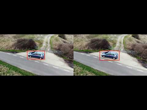
The final custom model provided good results when it was tested. Figure 4 shows the comparison between the two models on the same test video. ssd_mobilenet_v1_coco is on the left and the custom model is on the right.


Figure 4 - Comparison Between ssd_mobilenet_v1_coco and custom model
As seen in Figure 4 the trained model offers significant improvement in areas where ssd_mobilenet_v1_coco failed to detect the car. The model performed better than expected as only a small data set was used to train the model. Even with this improvement the model still isn’t perfect. It was only able to detect the car in 92% of the frames, Figure 5.
| Model | Average FPS | Percentage of Average Frames Detected | Confidence per Detected Frame |
|---|---|---|---|
| Custom Trained Model | 13.5 | 92.0 | 0.949 |
| ssd_mobilenet_v1_coco | 12.9 | 18.5 | 0.562 |
Figure 5 - Result Data Comparing Custom Model and ssd_mobilenet_v1_coco
The area which the custom model lacked accuracy was directly above the vehicle. This uncertainty is due to only having 6 images out of the 232 that feature the roof of cars. The issue could be rectified by simply adding more top view images. Lighting condition also affect the results. When the car is passing through a shaded area the model doesn’t always detect the vehicle as shown in Figure 6. Due to time constraints with the project it was decided to not spend more time developing the model as the time it would to take to achieve a small improvement wasn’t necessary and the training already accomplish the desired result.

Collecting more image for the training data set may yield better results. Also, relabelling the existing bounding boxes may improve the result as some of them were roughly done to speed up the labelling process, they may be too loose around the object. It’s worth looking in YOLOv3 Tiny as this CNN is designed to be extremely fast but at the cost of losing some accuracy.
[1] SSD: Single Shot MultiBox Detector https://arxiv.org/abs/1512.02325
[2] tzutalin/LabelImg https://github.com/tzutalin/labelImg
[3] datitran/Raccoon Detector Dataset https://github.com/datitran/raccoon_dataset/blob/master/xml_to_csv.py
[4] tenforflow/Tensorflow detection model zoo https://github.com/tensorflow/models/blob/master/research/object_detection/g3doc/detection_model_zoo.md
[5] Paperspace https://www.paperspace.com/