
![]()
Advanced Octave-Band and Fractional Octave-Band filter bank for signals in the time domain. Fully compliant with ANSI S1.11-2004 (Filters) and IEC 61672-1:2013 (Time Weighting).
This library provides professional-grade tools for acoustic analysis, including frequency weighting (A, C, Z), time ballistics (Fast, Slow, Impulse), and multiple filter architectures.
Now available on PyPI.
- 🚀 Getting Started
- 🛠️ Filter Architectures
- 🔊 Acoustic Weighting (A, C, Z)
- ⏱️ Time Weighting and Integration
- ⚡ Performance: Multichannel & Vectorization
- 🔍 Filter Usage and Examples
- 📏 Calibration and dBFS
- 📊 Signal Decomposition
- 📖 Theory and Equations
- 🧪 Testing and Quality
Option 1: From PyPI (Recommended)
Install PyOctaveBand directly using pip:
pip install PyOctaveBandOption 2: Cloning and Installing Clone the repository and install it manually:
git clone https://github.com/jmrplens/PyOctaveBand.git
cd PyOctaveBand
pip install .
Option 3: Git Submodule
Add PyOctaveBand as a dependency within your own git repository:
git submodule add https://github.com/jmrplens/PyOctaveBand.git
# Then install in editable mode to use it from your project
pip install -e ./PyOctaveBandAll core functionality can be imported directly from the pyoctaveband package.
| Name | Type | Description (Inputs) | Usage Snippet (Outputs) |
|---|---|---|---|
octavefilter |
function |
High-level analysis. • x: Signal array• fs: Sample rate [Hz]• fraction: 1, 3, etc. (Default: 1)• order: Filter order (Default: 6)• limits: [f_min, f_max] (Default: [12, 20000])• filter_type: 'butter', 'cheby1', 'cheby2', 'ellip', 'bessel' (Default: 'butter')• sigbands: Return time signals (Default: False)• detrend: Remove DC offset (Default: True)• calibration_factor: Sensitivity multiplier (Default: 1.0)• dbfs: Output in dBFS instead of dB SPL (Default: False)• mode: 'rms' or 'peak' (Default: 'rms')• show: Plot response (Default: False)• plot_file: Path to save plot (Default: None)• ripple: Passband ripple [dB] (for cheby1/ellip)• attenuation: Stopband atten. [dB] (for cheby2/ellip) |
spl, freq = octavefilter(x, fs, ...)• spl: levels [dB]• freq: frequencies [Hz]With sigbands=True:spl, freq, xb = octavefilter(x, fs, sigbands=True)• xb: List of filtered signals (one per band)Calibrated usage: spl, f = octavefilter(x, fs, calibration_factor=0.05) |
OctaveFilterBank |
class |
Efficient bank implementation. • fs: Sample rate [Hz]• fraction: 1, 3, etc.• order: Filter order• limits: [f_min, f_max] (Default: [12, 20000])• filter_type: Architecture name• show: Plot response (Default: False)• plot_file: Path to save plot (Default: None)• calibration_factor: Sensitivity multiplier• dbfs: Use dBFS (Default: False)• ripple: Passband ripple [dB]• attenuation: Stopband attenuation [dB] |
bank = OctaveFilterBank(fs=48000, fraction=3, order=6, filter_type='butter', show=True)spl, f = bank.filter(x, sigbands=False, mode='rms', detrend=True)• bank: Instance of the filter bank |
weighting_filter |
function |
Acoustic weighting. • x: Signal array• fs: Sample rate [Hz]• curve: 'A', 'C', or 'Z' (Default: 'A') |
y = weighting_filter(x, fs, curve='A')• y: 1D array of weighted signal |
time_weighting |
function |
Energy capture. • x: Raw signal array (squared internally)• fs: Sample rate [Hz]• mode: 'fast', 'slow', or 'impulse' |
env = time_weighting(x, fs, mode='fast')• env: 1D array of energy envelope (Mean Square) |
linkwitz_riley |
function |
Audio crossover. • x: Signal array• fs: Sample rate [Hz]• freq: Crossover frequency [Hz]• order: Any even number (Default: 4) |
lo, hi = linkwitz_riley(x, fs, freq=1000, order=4)• lo: Low-pass filtered signal• hi: High-pass filtered signal |
calculate_sensitivity |
function |
SPL Calibration. • ref_signal: Calibration signal• target_spl: Level of calibrator (Default: 94.0)• ref_pressure: Reference pressure (Default: 20e-6) |
s = calculate_sensitivity(ref_signal, target_spl=94.0)• s: Float (multiplier for pressure) |
getansifrequencies |
function |
ANSI Frequency generator. • fraction: 1, 3, etc. (Required)• limits: [f_min, f_max] (Default: [12, 20000]) |
f_cen, f_low, f_high = getansifrequencies(fraction=3)• f_cen: List of center frequencies [Hz]• f_low: List of lower edges [Hz]• f_high: List of upper edges [Hz] |
normalizedfreq |
function |
Standard IEC Frequencies. • fraction: 1 or 3 |
freqs = normalizedfreq(fraction=3)• freqs: List of standard center frequencies [Hz] |
Analyze a signal and get the Sound Pressure Level (SPL) per frequency band.
import numpy as np
from pyoctaveband import octavefilter

fs = 48000
t = np.linspace(0, 1, fs)
# Composite signal: 100Hz + 1000Hz
signal = np.sin(2 * np.pi * 100 * t) + np.sin(2 * np.pi * 1000 * t)

# Apply 1/3 octave filter bank
spl, freq = octavefilter(signal, fs=fs, fraction=3)

print(f"Bands: {freq}")
print(f"SPL [dB]: {spl}")

# OR: Import an audio file
from scipy.io import wavfile

# Load standard WAV file
fs, signal = wavfile.read("measurement.wav")

# Analyze
# Note: To obtain real-world SPL values, you must calibrate the input.
# See the [Physical Calibration](#physical-calibration-sonómetro) section.
spl, freq = octavefilter(signal, fs=fs, fraction=3)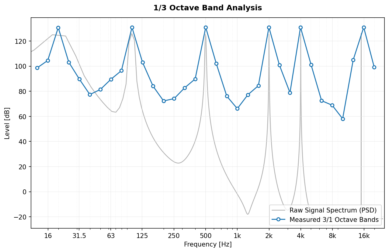
Example of a 1/3 Octave Band spectrum analysis of a complex signal.
PyOctaveBand natively supports multichannel signals (e.g., Stereo, 5.1, Microphone Arrays) using fully vectorized operations. Input arrays of shape (N_channels, N_samples) are processed in parallel, offering significant performance gains over iterative loops.
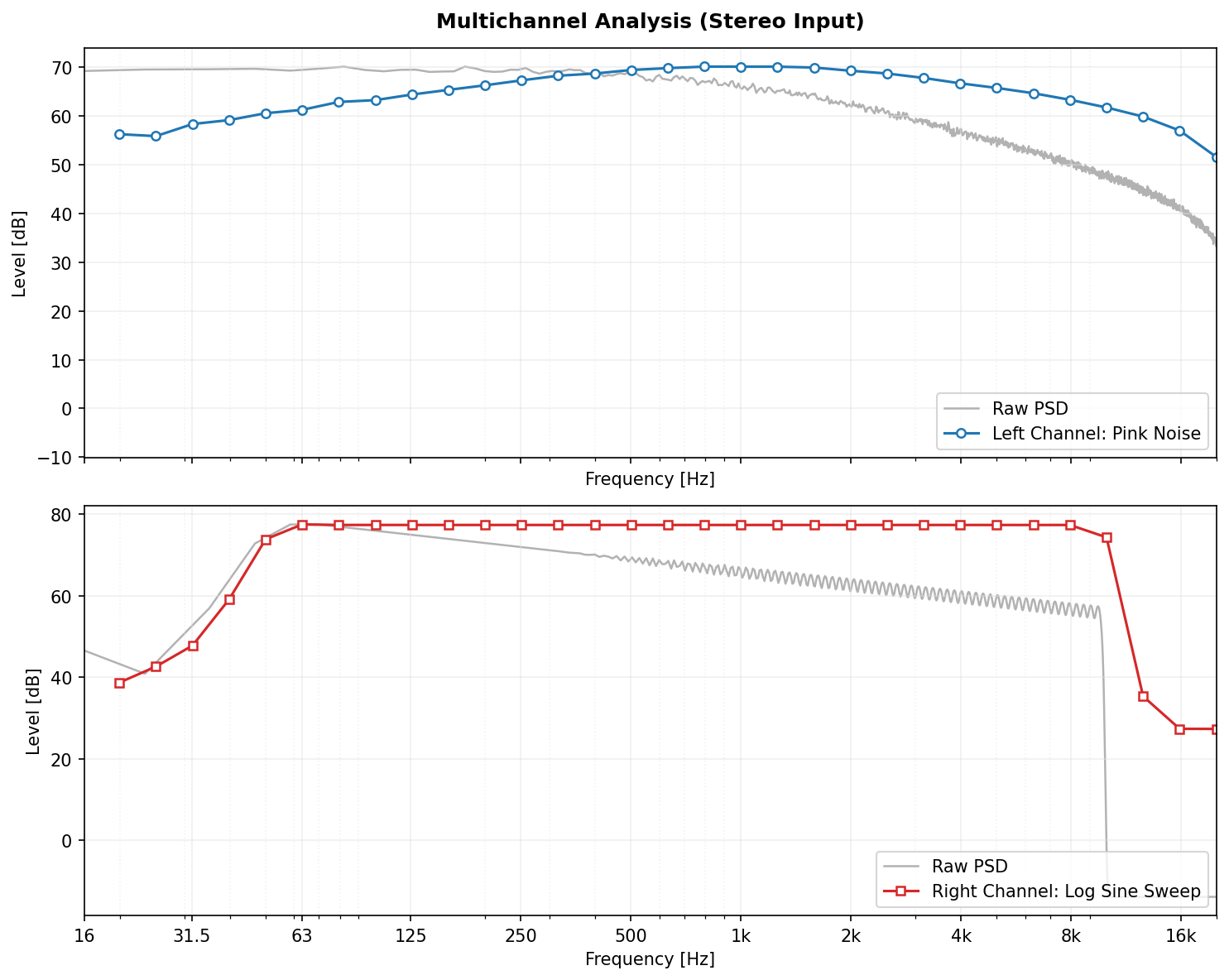
Simultaneous analysis of a Stereo signal: Left Channel (Pink Noise) vs Right Channel (Log Sine Sweep).
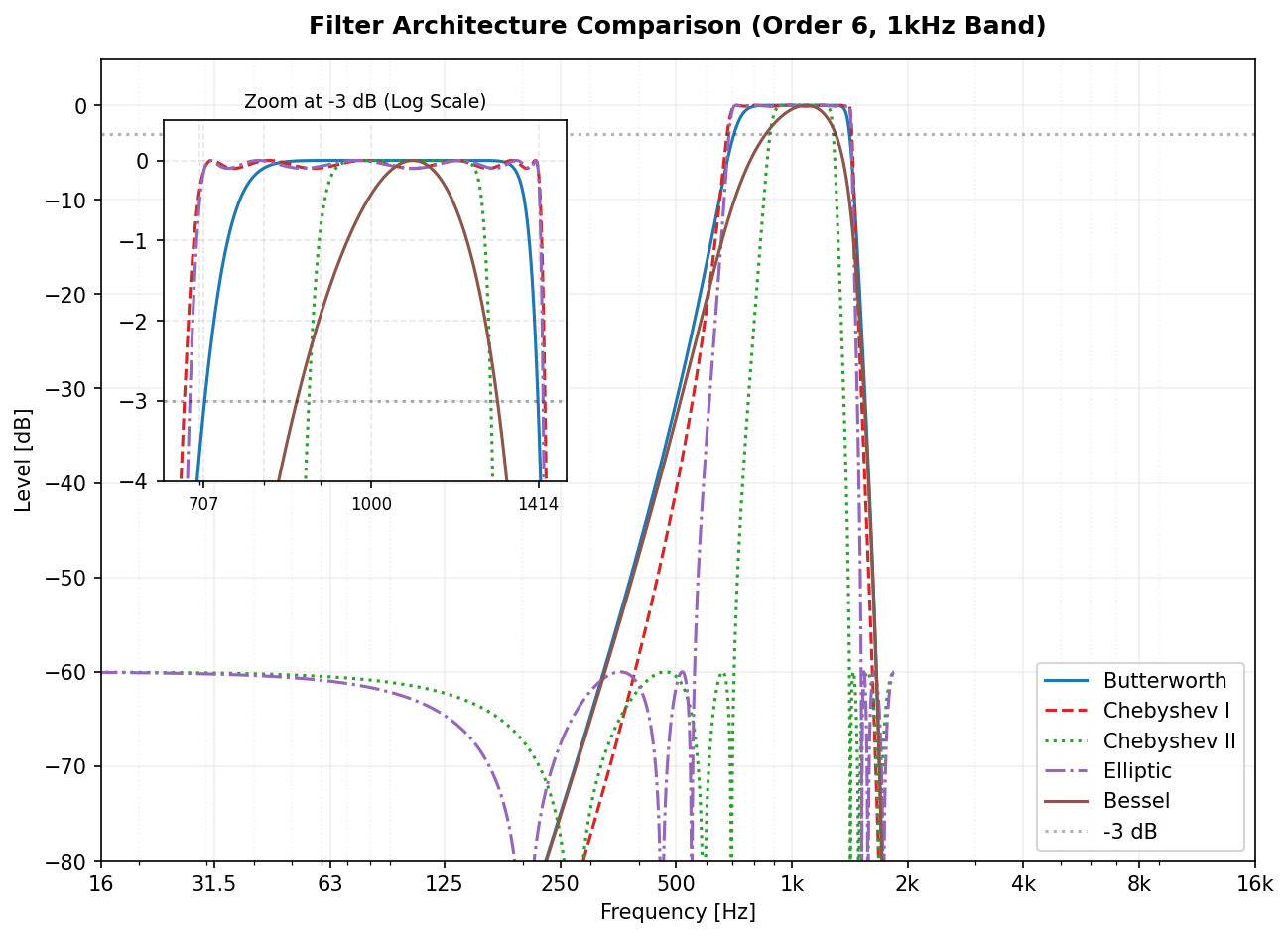
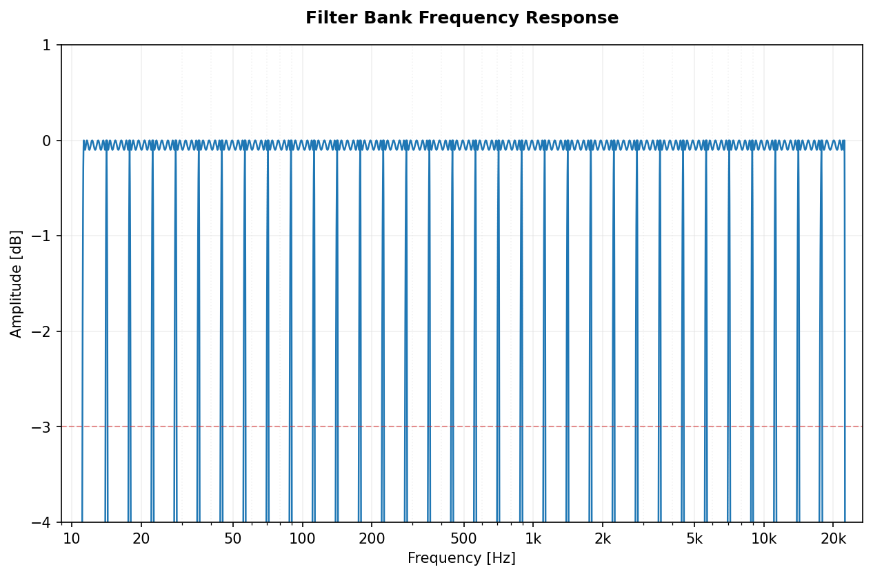
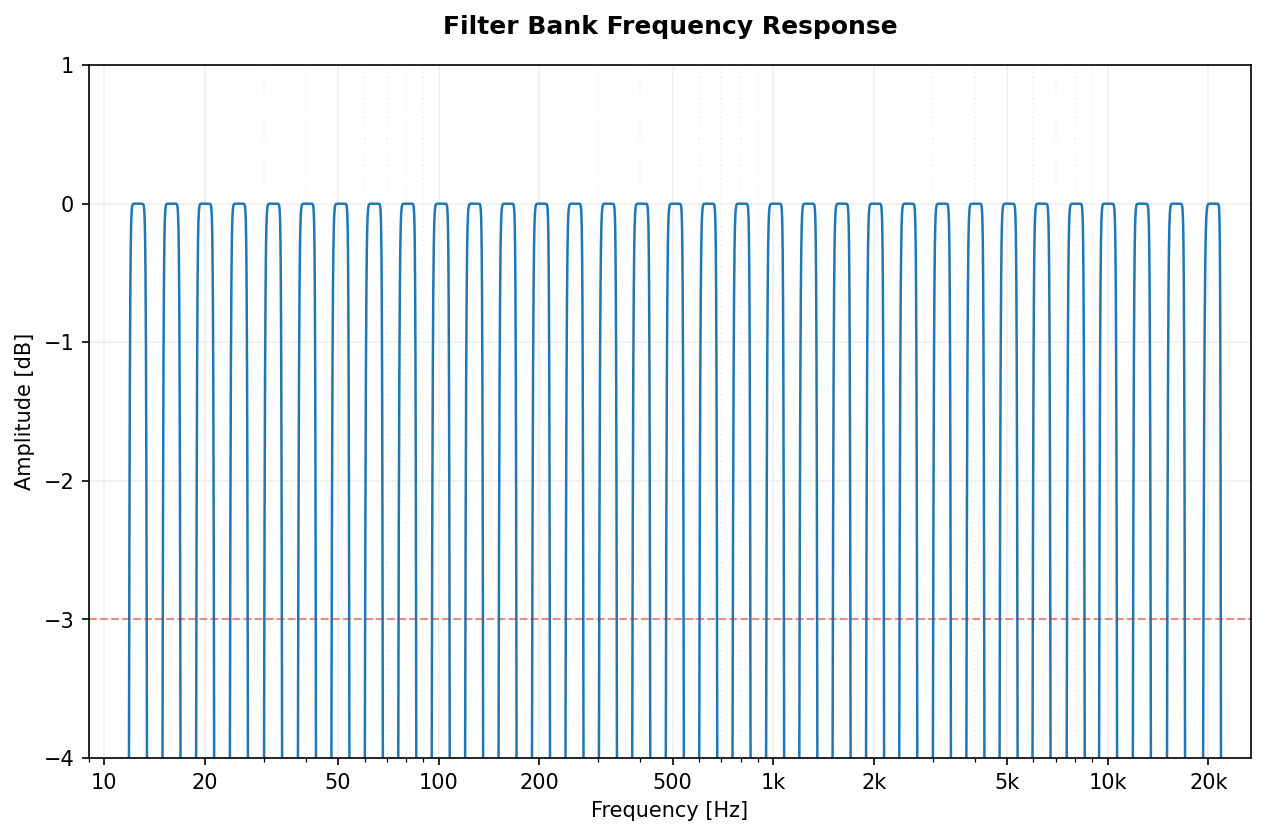
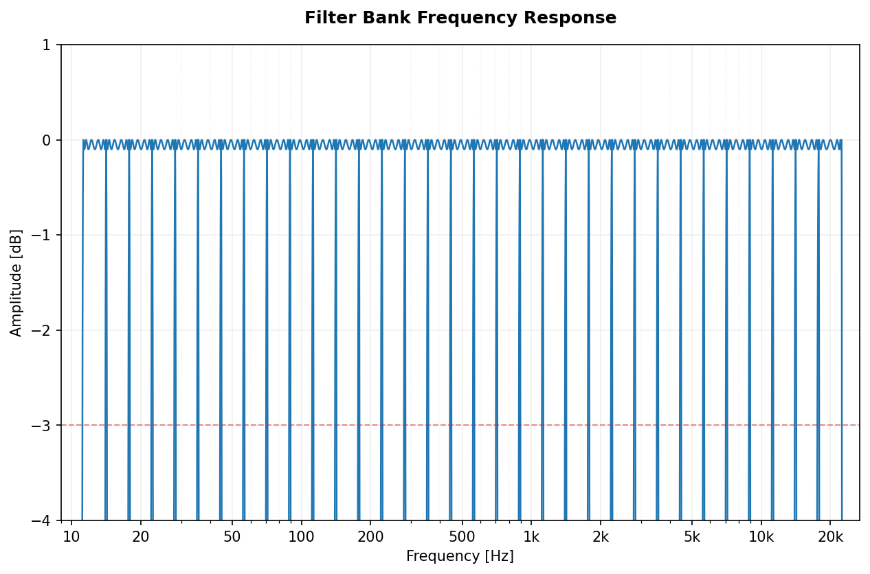
PyOctaveBand supports several filter types, each with its own transfer function characteristic.
We use Second-Order Sections (SOS) for all filters to ensure numerical stability. The following plot compares the architectures focusing on the -3 dB crossover point.
| Type | Name | Usage Example | Best For |
|---|---|---|---|
butter |
Butterworth | octavefilter(x, fs, filter_type='butter') |
General acoustic measurement. |
cheby1 |
Chebyshev I | octavefilter(x, fs, filter_type='cheby1', ripple=0.1) |
Sharper roll-off at the cost of ripple. |
cheby2 |
Chebyshev II | octavefilter(x, fs, filter_type='cheby2', attenuation=60) |
Flat passband with stopband zeros. |
ellip |
Elliptic | octavefilter(x, fs, filter_type='ellip', ripple=0.1, attenuation=60) |
Maximum selectivity. |
bessel |
Bessel | octavefilter(x, fs, filter_type='bessel') |
Preserving transient waveform shapes. |
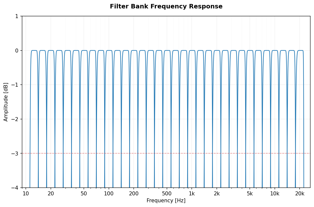
Full spectral view of the filter banks for Octave (1/1) and 1/3-Octave fractions.
| Architecture | 1/1 Octave (Fraction=1) | 1/3 Octave (Fraction=3) |
|---|---|---|
| Butterworth | 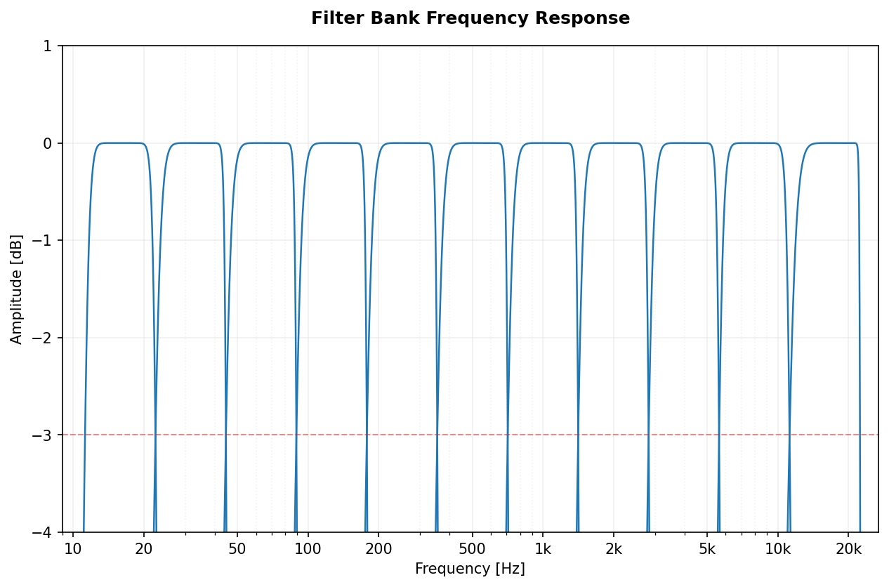 |
 |
| Chebyshev I | 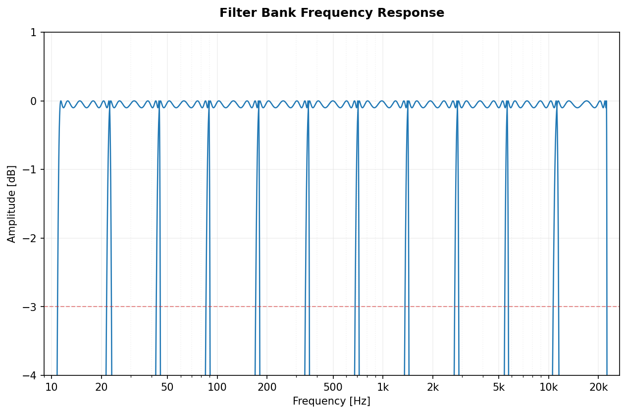 |
 |
| Chebyshev II | 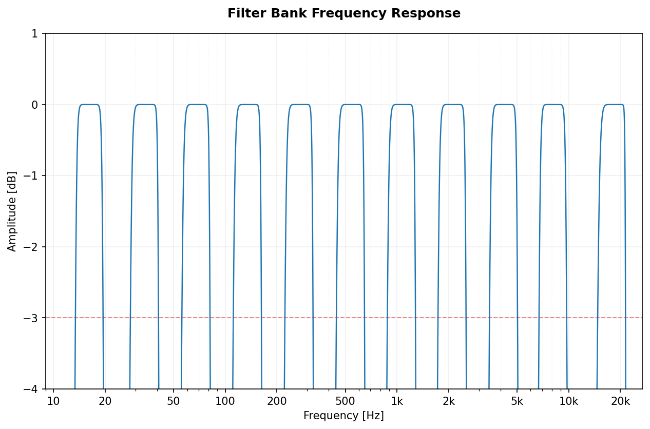 |
 |
| Elliptic |  |
 |
| Bessel | 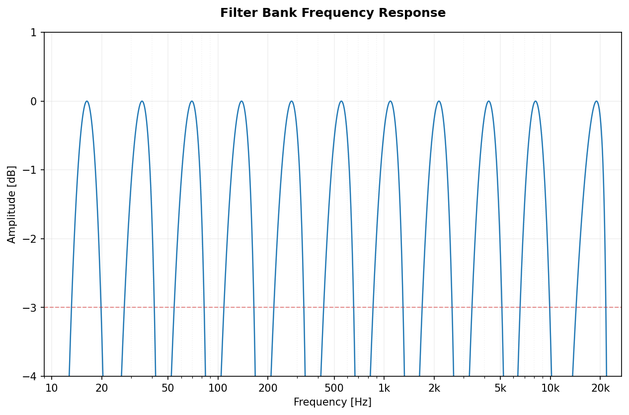 |
 |
Frequency weighting curves simulate the human ear's sensitivity.
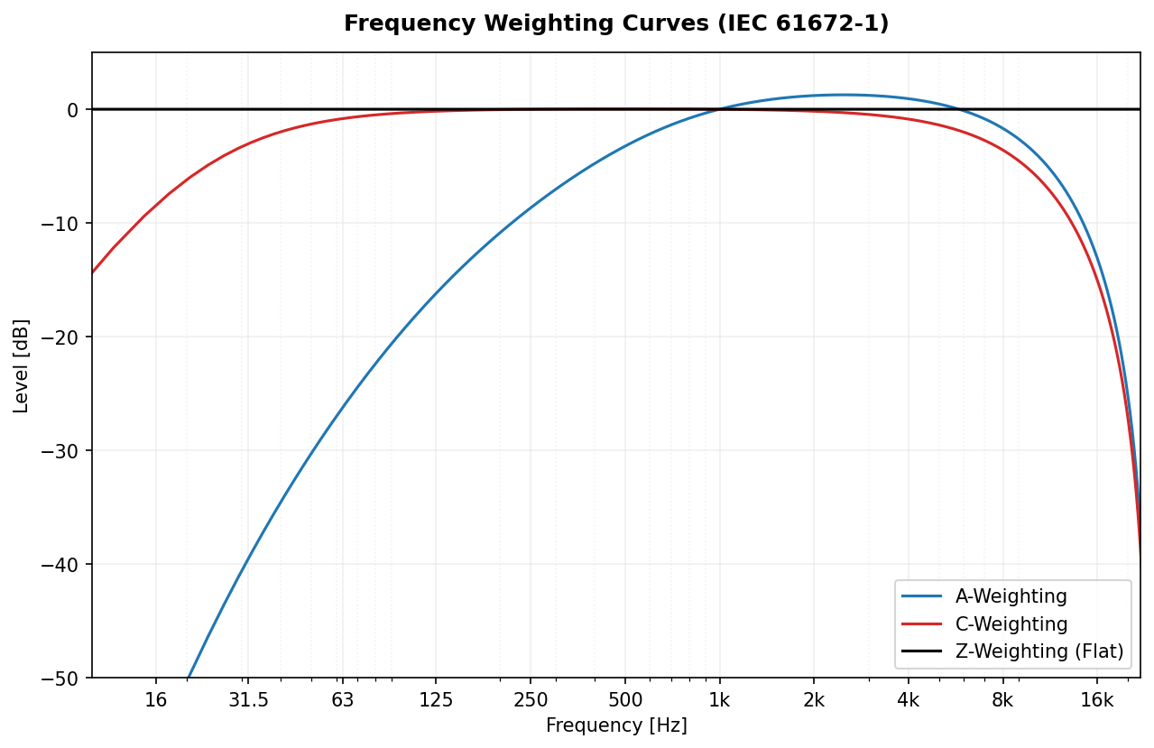
- A-Weighting (
A): Standard for environmental noise (IEC 61672-1). - C-Weighting (
C): Used for peak sound pressure and high-level noise. - Z-Weighting (
Z): Zero weighting, completely flat response.
from pyoctaveband import weighting_filter

# Apply A-weighting to the raw signal
weighted_signal = weighting_filter(signal, fs, curve='A')

# Apply C-weighting for peak analysis
c_weighted_signal = weighting_filter(signal, fs, curve='C')Accurate SPL measurement requires capturing energy over specific time windows. PyOctaveBand implements exact time constants per IEC 61672-1:2013.
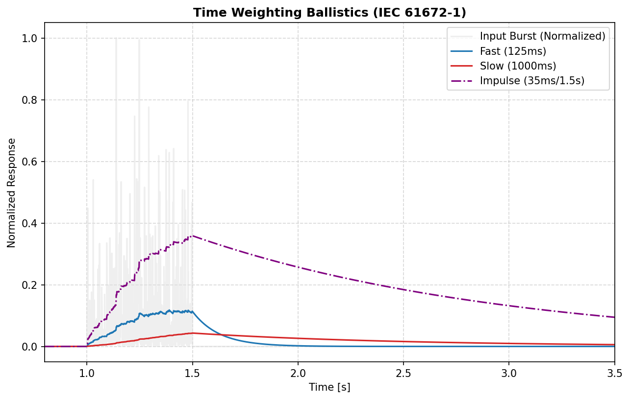
-
Fast (
fast):$\tau = 125$ ms. Standard for noise fluctuations. -
Slow (
slow):$\tau = 1000$ ms. Standard for steady noise. -
Impulse (
impulse): Asymmetric ballistics. 35 ms rise time for rapid onset capture, 1500 ms decay for readability.
from pyoctaveband import time_weighting

# Calculate energy envelope (Mean Square)
energy_envelope = time_weighting(signal, fs, mode='fast')
# dB SPL relative to 20μPa
spl_t = 10 * np.log10(energy_envelope / (2e-5)**2)The OctaveFilterBank class is highly optimized for real-time and batch processing. It uses NumPy vectorization to handle multichannel audio arrays (e.g., 64-channel microphone arrays) without explicit Python loops, ensuring maximum throughput.
from pyoctaveband import OctaveFilterBank

bank = OctaveFilterBank(fs=48000, fraction=3, filter_type='butter')

# Access computed properties
# bank.freq (center), bank.freq_d (lower), bank.freq_u (upper), bank.sos (coefficients)

# Process multiple signals efficiently
for frame in stream:
    # detrend=True (default) removes DC offset to improve low-freq accuracy
spl, freq = bank.filter(frame, detrend=True)This section provides detailed examples and characteristics for each supported filter architecture.
The Butterworth filter is known for its maximally flat passband. It is the standard choice for acoustic measurements where no ripple is allowed within the frequency bands.
from pyoctaveband import octavefilter
# Default standard measurement
spl, freq = octavefilter(x, fs, filter_type='butter')
Chebyshev Type I filters provide a steeper roll-off than Butterworth at the expense of ripples in the passband. Useful when high selectivity is needed near the cut-off frequencies.
# Selectivity with 0.1 dB passband ripple
spl, freq = octavefilter(x, fs, filter_type='cheby1', ripple=0.1)
Also known as Inverse Chebyshev, it has a flat passband and ripples in the stopband. It provides faster roll-off than Butterworth without affecting the signal in the passband.
# Flat passband with 60 dB stopband attenuation
spl, freq = octavefilter(x, fs, filter_type='cheby2', attenuation=60)
Elliptic (Cauer) filters have the shortest transition width (steepest roll-off) for a given order. They feature ripples in both the passband and stopband.
# Maximum selectivity for extreme band isolation
spl, freq = octavefilter(x, fs, filter_type='ellip', ripple=0.1, attenuation=60)
Bessel filters are optimized for linear phase response and minimal group delay. They preserve the shape of filtered waveforms (transients) better than any other type, but have the slowest roll-off.
# Best for pulse analysis and transient preservation
spl, freq = octavefilter(x, fs, filter_type='bessel')
Specifically designed for audio crossovers. Linkwitz-Riley filters (typically 4th order, but any even order is supported) allow splitting a signal into bands that, when summed, result in a perfectly flat magnitude response and zero phase difference between bands at the crossover.
from pyoctaveband import linkwitz_riley
# Split signal into Low and High bands at 1000 Hz
low, high = linkwitz_riley(signal, fs, freq=1000, order=4)
# Reconstruction: low + high == signal (flat response)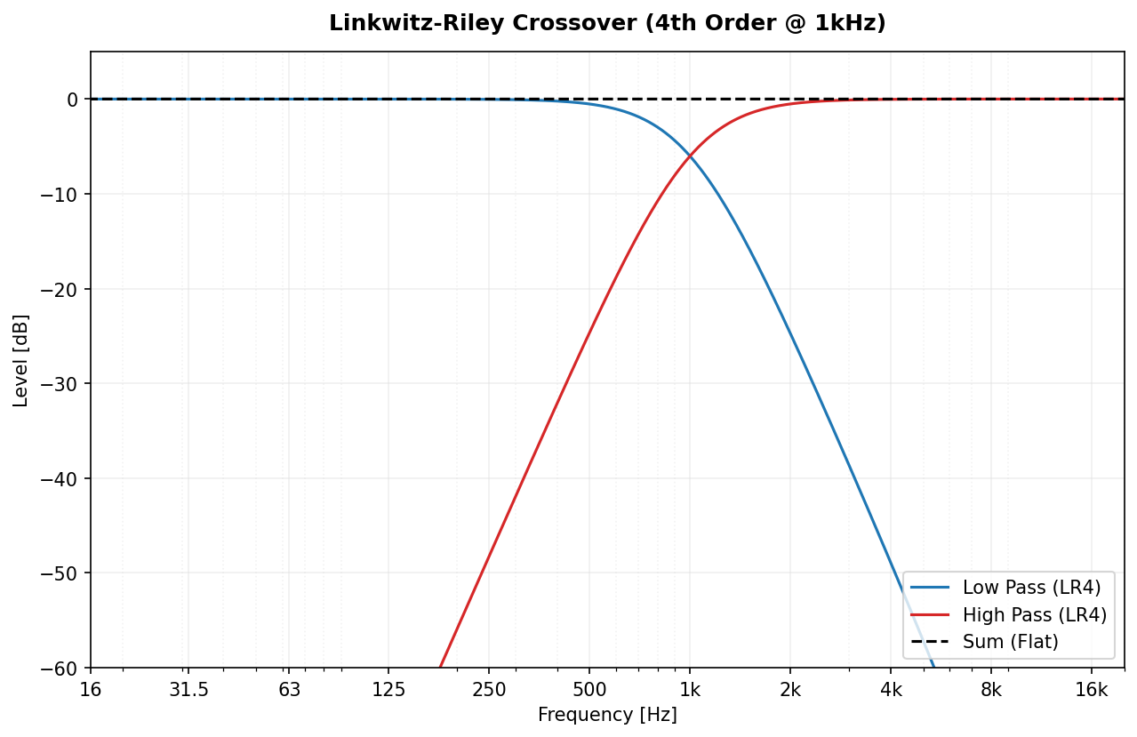
PyOctaveBand can return results in physical Sound Pressure Level (dB SPL) or digital decibels relative to Full Scale (dBFS).
To get accurate SPL measurements from a digital recording, you must first calculate the sensitivity of your measurement chain using a reference tone (e.g., 94 dB @ 1kHz).
from pyoctaveband import octavefilter, calculate_sensitivity

# 1. Record your 94dB calibrator signal
# ref_signal = ... (your recording)

# 2. Calculate sensitivity factor
sensitivity = calculate_sensitivity(ref_signal, target_spl=94.0)

# 3. Apply calibration to your measurements
spl, freq = octavefilter(signal, fs, calibration_factor=sensitivity)
# Now 'spl' values are in real-world dB SPL!If you are working with digital audio files (e.g., WAV, FLAC) and want to analyze levels relative to Full Scale rather than physical pressure, you can use the dbfs=True parameter.
In this mode:
- 0 dBFS corresponds to a numeric signal level of 1.0 (RMS or Peak).
- Useful for analyzing headroom, digital mastering, or normalized signals.
# Assume 'signal' is normalized between -1.0 and 1.0
spl_dbfs, freq = octavefilter(signal, fs, dbfs=True)
# Results will be negative (e.g., -20 dBFS)PyOctaveBand supports two measurement modes to align with professional software like BK:
- RMS (
mode='rms'): Energy-based level (standard). - Peak (
mode='peak'): Absolute maximum value reached in the frame (Peak-holding).
# Measure peak-holding levels for impact analysis
spl_peak, freq = octavefilter(signal, fs, mode='peak')By setting sigbands=True, you can retrieve the time-domain components of each band. This allows for advanced analysis or comparing how different architectures (e.g., Butterworth vs Chebyshev) affect the signal phase and transient response.
import numpy as np
from pyoctaveband import octavefilter

# 1. Generate a signal (Sum of 250Hz and 1000Hz)
fs = 48000
t = np.linspace(0, 0.5, int(fs * 0.5), endpoint=False)
y = np.sin(2 * np.pi * 250 * t) + np.sin(2 * np.pi * 1000 * t)

# 2. Compare architectures (Butterworth vs Chebyshev II)
# Filter with Butterworth (default)
spl_b, freq, xb_butter = octavefilter(y, fs=fs, fraction=1, sigbands=True, filter_type='butter')

# Filter with Chebyshev II (flat passband, ripples in stopband)
spl_c2, _, xb_cheby2 = octavefilter(y, fs=fs, fraction=1, sigbands=True, filter_type='cheby2')

# 'xb_butter' and 'xb_cheby2' contain the time-domain signals per band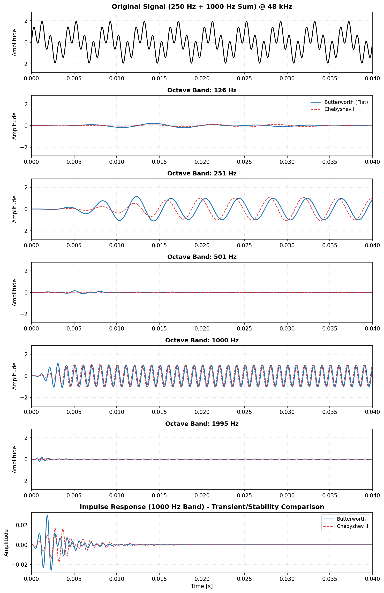
The plot compares the Butterworth (solid blue) and Chebyshev II (dashed red) responses. The bottom plot shows the Impulse Response, highlighting the differences in stability and transient decay.
Note
Why do the signals look shifted in time? Digital IIR filters (like Butterworth or Chebyshev) have non-linear phase responses, which results in frequency-dependent Group Delay. In the 250 Hz band, you can see that the Chebyshev II filter has a different propagation delay compared to the Butterworth filter. This is a normal physical property of these architectures: more aggressive frequency roll-offs usually come at the cost of higher group delay and phase distortion.
The mid-band frequencies (fm) and edges (f1, f2) use a base-10 ratio:
Mid-band:
(for odd b)
Band edges:
The library implements standard classical filter prototypes:
1. Butterworth: Maximally flat passband.
2. Chebyshev I: Equiripple in passband, steeper roll-off.
3. Chebyshev II: Inverse Chebyshev, equiripple in stopband, flat passband.
4. Elliptic: Equiripple in both, maximum selectivity.
5. Bessel: Maximally flat group delay (linear phase).
(Where
To ensure 100% stability across the entire audible spectrum (even at low frequencies like 16Hz with high sample rates), PyOctaveBand employs two critical strategies:
- Second-Order Sections (SOS): All filters are implemented as a series of cascaded biquads. This avoids the catastrophic numerical precision loss associated with high-order transfer functions (coefficients a, b).
- Multi-rate Decimation: For low-frequency bands, the signal is automatically downsampled (decimated) before filtering and upsampled afterwards. This keeps the digital pole locations far from the unit circle boundary, preventing oscillation and noise.
The A-weighting transfer function:
Implemented as a first-order IIR exponential integrator:
Where tau is the time constant (e.g., 125ms for Fast).
We maintain 100% stability and compliance through a rigorous test suite.
- Isolation Tests: Verifies that a pure 1kHz tone is attenuated by >20dB in the 250Hz and 4kHz bands.
- Weighting Response: Checks gains at 100Hz (-19.1dB for A) and 1kHz (0dB).
-
Stability (IR Tail): Analyzes the Impulse Response of every filter. Energy in the last 100ms must be
$< 10^{-6}$ to pass. -
Crossover Flatness: Verifies that the sum of Linkwitz-Riley bands has
$< 0.1$ dB deviation.
# Run full suite
pytest tests/

# Generate technical report
python scripts/benchmark_filters.pyJose M. Requena Plens, 2020 - 2026.