- To explore about introductory theories in image processing, which serves as a basic unit for studying computer vision.
- It also introduces fundaments of deep neural networks and its application to computer vision.
Briefly speaking, I implemented codes of
- Rotating, stitching of images
- Showing histogram of images
- Filters of images, specifically, gray filter, uniform mean filter, gaussian filter, sobel filter, laplacian filter, and unsharpMasking filter
- Salt and pepper noise, gaussian noise removals using median filter, mean filter, gaussian filters and etc.
- Edge/corner detection
- SIFT
- Affine/Hough transformation
- For more details about code, experiments, and analysis, please refer to technical report PDF.
- If you request me by yrs1107@gmail, I'll send you them. (Written in Korean)
This project requires:
- Visual Studio Community
- Version: 2019
- Library
- OpenCV 2.4.0
- tutorial pdf: OSP-Lec01-OpenCV_tutorial_for2.4.pdf
- OpenCV 2.4.0
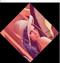
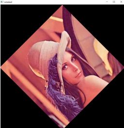
Rotation using interpolation method of bilinear (left) and nearest (right)
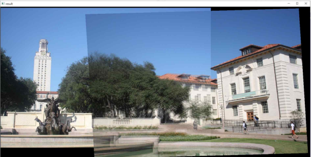
Stitching using inverse warping
ETC
- HW introduction: look at p.41 - 43 in pdf for more information : Rotating.Stitching.pdf
- LECTURE NOTES
- OSP-Lec00-Introduction.pdf
- OSP-Lec01-Fundamentals.pdf
- OSP-Lec02-Display.pdf
- OSP-Lec02-Display-Lab.pdf
Input image, grayscal image, and corresponding histograms

ETC
- HW introduction: look at p.34 - 44 in LECTURE NOTE pdf for more information
- LECTURE NOTES
- OSP-Lec03-Pixel.pdf
Mean Filter: according to filter size

Analysis
- 그림 4 에서와 같이 uniform mean filter을 거친 그림은 사진이 흐릿해져 보인다. 이 이유를 살펴보자면, filter을 통해서, 주변 값들의 평균을 output 픽셀 값에 넣으니, 원래는 선명했던 edge부분들이 다 평균화되면서 모두 옆의 주변 값들과 값이 얼추 맞춰졌기 때문이다.
- 그림 5와 그림 6을 살펴보자. 둘 다, zero-paddle 기법을 사용한 mean filter을 거친 이후의 output이다. 다만, 그림 5는 9x9 filter를, 그림 6은 25x25 filter를 사용하였다. 더 큰 filter size를 사용한 그림 6이 더 많이 blur된 모습을 볼 수 있다. 이유는 더 많은 주변 값들로 평균을 취했기 때문에 더 넓은 범위에서 평균화가 되어서이다. <br> 또한 주목할 점은, 그림 5와 그림 6의 boundary를 보면, 다른 기법을 취한 그림과 다르게 까맣다는 것을 확인 할수 있다. 그 이유는, zero-padding으로 image의 boundaries를 0으로 채워주었기 때문이다. 따라서 zero-paddle을 사용했을 때, 필터사이즈가 커짐에 따라, 이미지의 경계에서 0(검은색)이 되는 값들이 많아서 까만색 boundary를 형성한 것을 볼 수 있다.
Gaussian Filter: according to filter size

Analysis
- 그림 12의 오른쪽 그림과 그림 13을 보자. 각각 Gaussian filter(3x3, sigma = 1)을 거친 결과와 Gaussian filter (11x11, sigma = 1)을 거친 결과이다.
둘 다 sigma = 1 로 적용하였기 때문에 픽셀의 값은 중간에서 가장 높게 나타나며 sigma가 큰 경우보다 주변 값의 영향을 다소 적게 받는다. 따라서 smoothing 효과가 매우 자연스럽게 적용되었다. 그림 12보다 그림 13에서 필터사이즈가 컸으므로 아주 조금 더 smoothing 효과가 더 나타난 것을 확인할 수 있다.
그림 14을 보자. sigma = 5로 filter을 적용하였기 때문에, 그림 13의 같은 크기의 필터 사이즈((11x11, sigma = 1)를 가진 필터로 적용했을 때보다 더 많이 smoothing 효과가 나타났음을 확인할 수 있었다.
Sobel Filter: grayscale and RGB image

ETC
- HW introduction: look at p.34 - 38 in LECTURE NOTE pdf for more information
- LECTURE NOTES
- OSP-Lec04-Region.pdf
- Segmentation 프로그램 사용결과: Mean shift segmentation(프로그램 사용결과).pdf
Salt and Pepper Noise Removal: using Mean Filter

Analysis
그림 9, 10을 보자. 그림 10은 그림 9의 median filter을 거친 후 모습이다. 그림 9( noise : 20 % )는 앞선 그림 4( noise : 10% )보다 salt and pepper noise의 비율이 2배 높다. 따라서, 그림 10에서 볼 수 있듯이, median filter가 중간 중간에 죽여주지 못한 noise들이 다소 존재함을 볼 수 있다.
Gaussian Noise Removal: using Gaussian Filter

Analysis
그림 4는 Gaussian Noise가 추가된 그림이다. Salt and pepper noise가 추가된 그림보다 잔잔하게 noise가 깔렸다는 것을 확인할 수 있다. 그 이유는 salt and pepper noise는 극단적인 값인 0 또는 255만 가졌다면 Gaussian Noise는 Gaussian Distribution을 따르기 때문이다.
그림 5를 확인해보자. noise가 없어졌음을 확인할 수 있다. 하지만, Gaussian Filter은 Low pass Filter이기 때문에 edge부분들이 많이 소실되어 흐릿해졌음을 볼 수 있다.
ETC
- HW introduction
- look at p.27-31 in LECTURE NOTE [OSP-Lec05] pdf for more information (Noise Removal)
- look at p.51-53 in LECTURE NOTE [OSP-Lec06] pdf for more information (Segmentation)
- LECTURE NOTES
- OSP-Lec05-Restoration.pdf
- OSP-Lec06-Segmentation.pdf
Noise가 섞인 이미지를 Gaussian Filter를 적용한 후, Laplacian filter 적용

Analysis
- Gaussian filter의 sigma를 높여주었을 때의 효과에 대해 살펴보았다. sigma가 커졌다는 것은 옆 주변의 pixel 값들을 많이 죽이지 않는다는 뜻이다( blurring이 덜 됨) 따라서 그림4와 마찬가지로
짜잘짜잘한 노이즈들이 남아서 edge로 detect된 것을 확인할 수 있었다. (빨간색 동그라미 친 곳)
ETC
- HW introduction: look at p.40-42 in LECTURE NOTE pdf for more information
- LECTURE NOTES
- OSP-Lec07-Edge_Corner.pdf
Input images, I1 and I2 (left) and keypoint matching results (right)

ETC
- HW introduction: look at p.27-28 in LECTURE NOTE pdf for more information
- LECTURE NOTES
- OSP-Lec08-Descriptor.pdf
keypoint matching results with different threshold of ratio>ETC

Application: Stitching: SIFT + Affine Tranform

Analysis
- RANSAC을 적용하여 affine transformation을 한 결과, threshold를 해주기 때문에, inlier가 SIFT descriptor에서 얻은 keypoints의 개수보다 작다. 즉 affine transform T를 구할 때
사용하는 점의 개수가 훨씬 적다는 것이다. RANSAC은 SIFT에서 keypoints들을 찾을 때 제거하지 못한 outlier들을 효과적으로 제거할 수 있는 방법이다.
하지만, 필자가 RANSAC을 적용해보았을 때에는 오히려 RANSAC을 적용하지 않은 그림보다 RANSAC을 적용한 그림 3,4에서 좀 더 흔들림을 볼 수 있었다. 필자가 이에 대해서 생각해보았을 때는 이미 SIFT에서 ratio-thresholding과 cross-checking을 하면서 많은 outlier들이 제거되었기 때문이라고 생각을 하였다.
Hough Transformation using HoughlinesP function in OpenCV

Analysis
오른쪽 그림이 왼쪽 그림보다 accumulator에 나오는 수에 대해 threshold를 더 크게 잡았을 때이다. 이에 따라서, strict하게 line을 검출하였기 때문에 그림 1보다 더 적은 line이 검출되었음을 알 수 있다.
ETC
- HW introduction: look at p.28-31 in LECTURE NOTE pdf for more information
- LECTURE NOTES
- OSP-Lec09-Fitting.pdf
- Since files are too large to upload in github, I will share google drive link if you request
ETC
- HW introduction: look at LECTURE NOTE [OSP-Lec12-Backpropagation_MLP_practice.pdf] pdf for more information (especially p.14~16)
- LECTURE NOTES
- OSP-Lec11-Loss function.pdf
- OSP-Lec10-Deep learning_Intro.pdf
- OSP-Lec12-Backpropagation_MLP.pdf
- OSP-Lec12-Backpropagation_MLP_practice.pdf
- Since files are too large to upload in github, I will share google drive link if you request
ETC
- HW introduction: look at LECTURE NOTE [OSP-Lec14-CNN architecture-practice-v2.pdf] pdf for more information (especially p.22~31)
- LECTURE NOTES
- OSP-Lec13-CNN.pdf
- OSP-Lec14-CNN architecture.pdf
- OSP-Lec14-CNN architecture-practice-v2.pdf
- Since files are too large to upload in github, I will share google drive link if you request
ETC
- HW introduction: look at LECTURE NOTE [OSP-Lec15-Encoder_Decoder-practice-v2.pdf] pdf for more information (especially p.5~11)
- LECTURE NOTES
- OSP-More on deep learning.pdf
- OSP-Lec15-Encoder_Decoder.pdf
- OSP-Lec15-Encoder_Decoder-practice-v2.pdf