blendmpc

blendmpc implements four common ways of combining trajectory-optimization MPC with reinforcement learning: residual RL on top of an MPC controller (Johannink et al., 2019), learned value functions as MPC terminal costs (Bhardwaj et al., 2021), warm-starting the solver with a learned policy (Mansard et al., 2018), and collecting MPC rollouts to train imitation policies (DAgger-style; Ross et al., 2011). These patterns keep showing up in robotics papers as one-off implementations; here they are ordinary library components that work with Gymnasium environments, the Crocoddyl and acados solvers, and any RL library that consumes Gymnasium envs (the benchmarks use Stable-Baselines3).

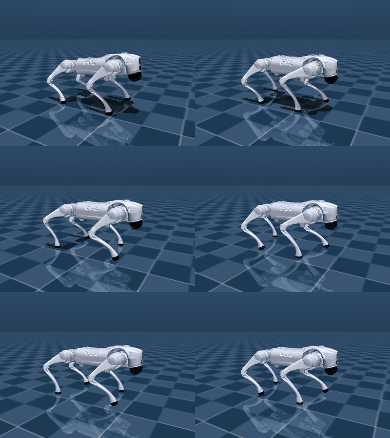
Unitree Go2 walking at 0.3 m/s under the whole-body gait MPC (CrocoddylCyclicMPC + Crocoddyl, ~3 ms per solve at 50 Hz, MuJoCo plant). Rendered by benchmark/quadruped_trot/render.py.

Residual SAC on Pendulum-v1 with the plant mass 40% higher than the MPC's model. The residual agent starts near the MPC baseline and skips the initial crash phase of SAC from scratch. Script: benchmark/residual_pendulum.

Installation

pip install "blendmpc[crocoddyl]"

Add the quadruped extra for the Go2 tasks (MuJoCo + robot_descriptions). Crocoddyl installs from wheels; the acados backend additionally needs the acados C library and is skipped everywhere (tests included) when absent. For development:

git clone https://github.com/assawayut/blendmpc && cd blendmpc
pip install -e ".[crocoddyl,test]"

Usage

import gymnasium as gym
import numpy as np

from blendmpc.blends import ResidualMPCEnv
from blendmpc.envs.pendulum import make_pendulum_problem, obs_to_state
from blendmpc.solvers.crocoddyl import CrocoddylMPC

mpc = CrocoddylMPC(lambda x0: make_pendulum_problem(x0, horizon=30))
env = ResidualMPCEnv(gym.make("Pendulum-v1"), mpc, obs_to_state)

obs, _ = env.reset(seed=0)
done = False
while not done:
    obs, reward, terminated, truncated, info = env.step(np.zeros(1))
    done = terminated or truncated

env is a normal Gymnasium environment whose action is a correction added to the MPC, so the zero action above reproduces the plain controller (it swings the pendulum up on its own). Training an agent on it works as usual:

from stable_baselines3 import SAC
SAC("MlpPolicy", env).learn(total_timesteps=15_000)

See examples/ and the documentation for the other components.

Components

• ResidualMPCEnv — Gymnasium wrapper implementing u = clip(u_mpc + a_rl). Useful when the MPC's model is wrong in ways that are hard to write down (payload mass, friction, cable drag). Keep the residual authority at 1.0 unless you have a reason not to; a bounded correction cannot beat the base controller's ceiling.
• make_learned_terminal / with_learned_terminal — put a learned cost-to-go V(x) at the terminal node of a Crocoddyl problem, so a short horizon behaves like a long one. Takes analytic grad_fn/hess_fn (e.g. torch autograd); finite differences on a float32 network are too noisy to use.
• PolicyWarmStartMPC — roll out a policy to initialize the solver on cold starts. With compare_with_default=True it solves from both the policy seed and the solver's own init and keeps the cheaper solution.
• collect_expert_dataset — run the MPC in closed loop and record (obs, u_mpc) pairs for behavior cloning. Pass policy= to let the student drive while the MPC labels (DAgger-style).

Backends (CrocoddylMPC, AcadosMPC) share one interface, MPCPolicy.solve(x0, us_init, xs_init); the base class turns it into a receding-horizon controller with warm-start shifting. Components only see that interface, so adding a backend does not touch them.

Benchmarks

Each component has a benchmark under benchmark/ that reruns in minutes on a CPU. Numbers below are mean return over 15 fixed evaluation episodes of the pendulum swing-up (higher is better; a failed swing-up is roughly -1500).

	result
MPC with 40% mass error	-629
+ residual SAC, 15k steps	-273
SAC from scratch, 15k steps	-236 (first ~2.5k steps at ~-1450)
MPC, horizon 30	-320, 14/15 swing-ups
MPC, horizon 8	-1536, 0/15
MPC, horizon 8 + learned V	-414, 14/15 (15/15 with a value-iteration V)
BC student of the MPC	-423 at 25x lower latency (0.6 ms → 24 µs)

The same residual pattern on a real robot morphology — whole-body MPC on the Unitree Go2 (37-dimensional state, 12 torques, 50 Hz, ~3 ms per solve), carrying roughly its rated payload unmodeled (benchmark/quadruped_balance):

	return
MPC, true-mass model	-2.49
+ residual SAC, 60k steps	-3.50 (best seed -2.69)
MPC, nominal model	-5.67
SAC from scratch, 60k steps	-12.79

And with a gait: CrocoddylCyclicMPC advances a periodic contact schedule through the receding horizon (ShootingProblem.circularAppend); with a velocity command the swing-foothold schedule and base reference advance too, and the robot walks (0.2–0.3 m/s tracked to within a few mm/s; the envelope ends near 0.4 m/s). The benchmark below trots in place while carrying three times its trunk mass unmodeled (benchmark/quadruped_trot). Here the learned residual ends twice as good as the true-model controller — the remaining error is contact timing, which no rigid-body parameter can fix:

	return
+ residual SAC, 60k steps	-5.81
Trot MPC, true-mass model	-11.79
Trot MPC, nominal model	-24.12

The gait also distills (benchmark/quadruped_distill): a phase-conditioned MLP clone of the trot MPC keeps the full gait (identical airborne fraction, 5/5 survival, return within 8%) at 28 µs per action — 142× faster, deployable at multi-kHz rates with no solver on board.

Some observations from producing these, written up in the benchmark READMEs:

• What looks like the solver getting stuck in a local minimum is often the objective itself: from a hanging start, staying down genuinely costs less than swinging up over a 1.5 s horizon. Warm-start seeding cannot fix this; a terminal value function can.
• Warm-starting a receding-horizon MPC from its own shifted solution can lock in whatever the first solve found. A small nonzero cold-start control gets out of stationary points; re-seeding from a policy at every step made closed-loop performance worse in all runs.
• One round of MSE DAgger made the distilled student worse, not better. The expert is close to bang-bang, so student-visited states get contradictory labels and the regression averages them into torques that mean nothing.
• The terminal value function has to be trained in the same cost units the OCP uses. Fitting it to the environment's reward (differently scaled, kinked at the hanging angle) quietly breaks it.
• On the quadruped, residual authority works the other way around from the pendulum: large residuals let exploration noise knock the robot over and training data becomes mostly falls. And per-step rewards that are tiny against SAC's entropy bonus quietly pay the policy to stay noisy — scale training rewards before blaming the blend.
• The pendulum's learned-terminal-cost win does not transfer to the quadruped: with a gait schedule imposing the contact sequence, an 8-node window trots just as well as a full-cycle one at a quarter of the solve time, and the balance task is better at horizon 2 than 25. Terminal value functions fix discovered long-horizon structure, not scheduled structure.

Related projects

• mpcrl and mpc4rl treat the MPC itself as the function approximator and let RL tune its parameters (Gros & Zanon). blendmpc keeps the controller and the policy separate instead; the two approaches are complementary.
• Crocoddyl and acados do the actual optimization.

Roadmap

Planned: a PyPI release, faster gaits, and lateral/turning commands. Contributions are welcome, in particular new solver backends and patterns from papers you want reusable — see CONTRIBUTING.md.

Citing

If you use blendmpc in your research, please cite it via CITATION.cff (the "Cite this repository" button on GitHub).