Numerical Solution for the Thomson Problem

A numerical approach to 3D (sphere) Thomson problem for N particles.

Abstract

The Thomson problem tries to determine the configurations of N electrons constrained on a unit sphere that results in the minimum electrostatic potential energy. A purely geometrical counterpart of this problem can be described as a problem that tries to determine the configuration of N points on the surface of a unit sphere that results in the maximization of minimum distances between the points. The exact solutions to the Thomson problem are known for a handful of cases. However, so far (as of 2023-01-20), there is no generalized solution to the Thomson problem for any number of electrons (or points) on a unit sphere.

There are likely a number of numerical solution algorithms that can find approximate solutions for the Thomson problem for a given number of electrons. I merely wanted to present a rather simple approach I developed on my own.

Numerical Solution

An iterative method is used. Initially, N electrons are placed on the unit sphere randomly.

    # Initialize electrons at random positions on a unit sphere
    # that is centered at position (0,0,0).
    electrons = []
    for i in range(n):
        new_pos = vec3()
        new_pos.x = random.uniform(-1, 1)
        new_pos.y = random.uniform(-1, 1)
        new_pos.z = random.uniform(-1, 1)
        new_pos = new_pos.normalized()
        
        new_electron = electron(new_pos)
        electrons.append(new_electron)

Then, the electrons are allowed to apply accelerations on each other via the Coulomb force. The exact magnitude of the forces are not calculated according to the constants used for electron charge - the magnitude multiplier of the forces do not have any effect on the minimum energy configuration.

        current_electron_accels = []
        # we will calculate acceleration of each electron...
        for e in electrons:
            total_electron_accel = vec3(0, 0, 0)

            # ...due to each electron...
            for e2 in electrons:
                
                # ...that is not the electron we are
                # currently calculating the acceleration of.
                if not e == e2:
                    total_electron_accel += e.calc_accel(e2)

            current_electron_accels.append(total_electron_accel)

The calculated accelerations are then used to modify the velocities of the electrons on the unit sphere. However, the velocity vectors are reduced to their 90% and an optional relaxation factor is applied to ensure convergence. Otherwise, the electrons may move back-and-forth around the minimum acceleration points where the actual solutions might be, but the solution might not converge due to the constant "swinging".

        # Accelerations have been calculated. Now, update their velocities.
        for idx_e in range(len(electrons)):
            e = electrons[idx_e]
            # apply 10 percent "drag" so that electrons lose velocity over steps and do not bounce around their lowest energy points
            e.update_vel((current_electron_accels[idx_e] - current_electron_accels[idx_e] * 0.9) * relaxation_factor)

            # limit velocity components so that the electrons only move on
            # the surface of the sphere
            radial_vel = e.vel.dot(e.pos.normalized())
            e.vel = e.vel - e.pos.normalized() * radial_vel

        # Velocities are updated. Now, update positions.
        old_positions = []
        new_positions = []
        for e in electrons:
            old_positions.append(e.pos)
            e.update_pos()
            e.pos = e.pos.normalized() # limit movement domain to sphere surface
            new_positions.append(e.pos)

Convergence is checked by looking at whether the positions of electrons are stable below a certain specified tolerance.

        # check for position convergence
        convergence_list = []
        for idx_pos in range(len(old_positions)):
            old_pos = old_positions[idx_pos]
            new_pos = new_positions[idx_pos]

            convergence_list.append((new_pos - old_pos).mag())

        converged = all(i < tolerance for i in convergence_list)

The tolerance and relaxation values must be used carefully. A relaxation factor too small or a tolerance too large may falsely trigger the convergence flag. In addition, it is always a good idea to examine the resulting 3D plot for a sanity check.

Validation & Solutions:

The exact solutions for N=6 and N=12 are known. The numerical solutions were obtained as follows:

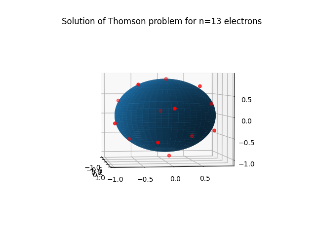
The solution for N=13 is not known exactly, but the following result was obtained via the numerical approach described above: