LIDAR Robot Tracking Algorithm

LIDAR simulator and visualizer along with an algorithm to calculate the center of robots through LIDAR data.

The program allows you to set down a LIDAR, customize the robot cross-section that the LIDAR sees, customize the path the robot travels along, and then simulates various algorithms tracking the robot as it moves.

2023-05-06.19-50-20.mp4

The pink line is the naive averaging algorithm, and the blue line is the algorithm I developed.

Run python playground.py while in the project directory to start the program.

The Problem

I was tasked with exploring the problem of tracking opposing robots using a LIDAR mounted on an robot. The LIDAR can measure the distance of objects away from the robot in a multitude of different directions. Using this data, a point cloud of what the robot “sees” around it can be extracted. The problem with trying to track other robots with this is that LIDAR data says nothing about the geometry of the side of objects not exposed to the LIDAR, and the LIDAR shoots beams in a plane, so the point clouds only give the geometry of a cross-section of other robots. Due to physical constraints, the LIDAR had to be mounted up high on our robot. The base of the robots we were dealing with were usually square, but higher up, there is no garuntee of what shape we will see. Thus, the cross sections the LIDAR would see would be highly variable, sometimes discontinuous, and may not reflect the geometry of the robot as a whole.

Suppose that you isolate some points that you can associate to be a part of an opposing robot. The easiest way to estimate the center of this robot is to take the average of these points. The problem with this is that the estimate will be biased towards the LIDAR, since the point cloud consists only of points that are exposed to the LIDAR. The backs of opposing robots, for example, will not be present in the point cloud.

Preliminary Ideas in Finding a More Accurate Estimate

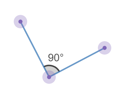
One idea I had before being notified that the LIDAR had to be mounted high up is that we would could take advantage of the usually square bases of opposing robots. If the LIDAR was mounted lower, the cross-sections we would pick up would be the square bases. From most angles, the LIDAR would be able to pick up two faces of the square. If you are able to fit two lines to the point cloud (one for each face), you can then use a little geometry to calculate the center of the sqaure, and thus the robot.

Example two faces that the LIDAR may pick up:

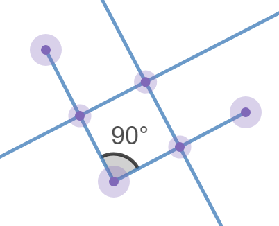
Construct the perpendicular bisectors of each face and their intersection is the location of the center:

However, this idea wouldn't work since as mentioned before, the LIDAR had to be mounted up high.

Initially, I was inclined to use data over multiple LIDAR scans to construct a better estimate. One idea I had was to build a "profile" of opposing robots. As time progressed and more data comes in, the LIDAR might see opposing robots from different angles and be able to stitch together the full cross-section. Then, whenever the LIDAR picked up a part of the opposing robot, we could try to match the full cross-section to the single part we picked up to get the exact positioning of the entire cross-section in that moment of time. Finally, simply average all the points to approximate the center (this is better now that the entire cross-section is represented in the point cloud).

This idea of stitching together scans and matching the stitched point cloud to the single part point cloud can be achieved through what is called scan matching.

Another idea I had using scan matching was to match the two LIDAR point clouds of an opposing robot over a time step to figure out the rotation and translation of the opposing robot's point cloud in that time step (taking into account the motion of the LIDAR itself of course). I thought that this might be able to help us deduce the center, but after doing a little bit of math, it actually turns out that with this information, every single point in the plane can be a possible candidate for the center of the robot (every point in the plane corresponds to a different displacement of the robot's center over the time step).

Obviously every point in the plane can't be a candidate for the center. The robots we were dealing with are finite in size. The center can't be thousands of miles away. This line of thinking led me to finding a very nice solution to this problem.

I ended up abandoning my earlier scan matching approaches since the solution I found was much less technical, probably more computationally performant, and I wasn't sure how well scan matching would work with robot point clouds since they consist of a relatively small amount of close together points.

High-Level Overview of the Algorithm I Developed

The robots that we are tracking are in the VEX Robotics competition. These robots need to fit within a certain sizing cube. This coresponds to the cross sections we pick up needing to fit within a certain square. We can reasonably assume that robots are able to be placed in the sizing cube such that their center lines up with the center of cube (disregarding the vertical coordinate).

Thus, first find every single square (including rotated ones) of regulation size that fit around the opposing robot's point cloud. The center of one of these squares is the center of the robot by our previous assumption. Take these squares, extract the $(x, y)$ locations of their centers, and then combine that with the rotation of each square to create the set of all possible candidates for the current $(x, y, \theta)$ state of the robot.

Finally, find the average x and average y of all the $(x, y, \theta)$ possible candidate states, ascribing equal weight to each. Note that this means that if a possible $(x, y)$ location of the center of the robot has more possible rotations that the robot could be in, it will have a higher weight in the average. We now have an estimate of the center of the opposing robot.

This algorithm is interesting, since normally we are concerned with fitting robots inside of the sizing cube, but now, we are concerned with fitting the cube around the robot. A bit of a reversal of roles.

Details of the Algorithm

I was a bit hand-wavy with "find every single square (including rotated ones) of regulation size that fit around the opposing robot's point cloud." How do we go about actually doing this?

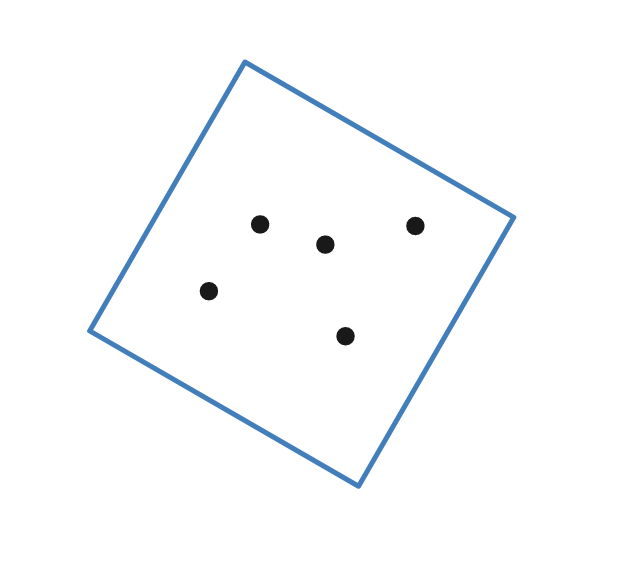
First, let "valid square" mean a square of regulation size that contains all the points of the opposing robot's point cloud.

Simple Case

Let's break down the problem into a simpler one. Suppose that we cannot rotate the square, so it must stay upright. Through some quick experimentation, we can visually see what all of the valid squares are by sliding around the square:

If the highest point is below the top edge of the square, the left-most point is to the right of the left edge of the square, etc., then the square is valid.

Furthermore, we can see that the centers of all of these valid squares form a rectangle:

The center of the rectangle can't go any more right when the left side of the square strikes the left most point, so the x-coordinate of the right side of the rectangle is $L.x + \frac{S}{2}$ where $L$ is the left most point and $S$ is the side length of the square.

Similar logic can be used to derive the other coordinates of this rectangle, and of course, more rigorous logic can be used to prove the center of the square is within this rectangle if and only if the square is valid.

Reducing to Simple Case

Say now that we want to find all valid squares of a certain rotation, and more importantly, their centers:

We can rotate the entire problem so that the square is upright:

Solve for all the centers of valid upright squares there:

Rotate back to get the solution:

The rotations can be performed using rotation matrices

(There are multiple ways to think of this process such as changing coordinates to a rotated coordinate system and then performing identical reasoning as the simple case)

So finally, we can simply repeat this procedure for all possible rotations of valid squares. Note that due to symmetry, we only need to check for rotations from 0 to 90 degrees. Of course, there are infinite such rotations, so one can simply consider a reasonable finite amount of rotations between 0 to 90.

Performing Averaging Math

We can now find all possible $(x, y, \theta)$ candidates for the center of the opposing robot (at least an approximation of the space). How do we get the average $(x, y)$?

The great thing about averages is that you can calculate them by taking the weighted average of averages of a partition:

$$Avg = \frac {\iiint_V{(x, y) \ dv}} {|V|} = \frac{\sum_i{\iiint_{V_i}{(x, y) \ dv}}} {|V|} = \frac{\sum_i{\frac{\iiint_{V_i}{(x, y) \ dv}} {|V_i|} \cdot |V_i|}} {|V|} = \frac{\sum_i{{Avg}_i \cdot |V_i|}} {\sum_i{|V_i|}}$$

Where $|V|$ denotes volume the volume of $V$ and $\{ V_i \}$ is a partition of $V$

Since our (x, y, theta) space will actually consist of rectangular cross sections at a finite amount of theta from 0 to 90 as mentioned before, we will use the above formula, but with double integrals and regions instead of volumes:

$$Avg = \frac{\sum_i{{Avg}_i \cdot |R_i|}} {\sum_i{|R_i|}}$$

where $i$ is an index representing a certain rotation of the valid squares, $R_i$ is the rectangle of all valid (x, y) centers for the certain rotation, and ${Avg_i}$ is the average of that rectangle.

$Avg_i$ is simply the center of $R_i$, and $|R_i|$ can be computed with length times width.

So now, we can compute the average and get our estimate of the opposing robot's center.

The implementation can be seen in the algorithms.py file.

How is its Accuracy?

As you can see in the video above, the algorithm has an average error lower than the naive averaging algorithm (from experimentation around 2x less), but its estimations are much more erratic. When the LIDAR is able to see a large corner, there are typically very few valid squares, so the algorithm becomes very accurate. However, when the LIDAR is only able to see one face, the algorithm devolves to the naive averaging algorithm. Additionally, when the features of the robot cross-section are very close together, the algorithm isn't much better than the naive averaging approach. Certain cross-sections make this algorithm perform extremely well, and others, not so much.

There are some parameters than can be tuned in the algorithm, such as the amount of valid square rotations between 0 to 90 that are checked, that will also change the accuracy of the algorithm.